This page is a preview of some ideas from Ch 4.

A linear transformation is a function from one vector space to another (that obeys a few rules..). You saw very simple examples in Calculus, such as the function f(x) = 2x. You can check it obeys one of the rules - that f(0) = 0. It may surprise you that f(x) = 2x + 1, for example, is not a linear transformation. It doesn't obey this basic rule!

The first computer graphic shows the effect of the transformation, f(x) = 2x. We say it stretches, scales, or dilates the line. Click on your browser's refresh or reload button to watch it again.

The green bar in the picture is the real line, the vector space R¹. The silver ball is the vector 0, which doesn't move. The short yellow bar is the interval S = [-1,1]. After doubling all these numbers, the interval grows to [-2,2]. This new set can be called "f(S)".

Disclaimers: There is nothing special about the interval [-1,1]. I just needed a second color besides green to show the effect.

Also, the animation really shows a sequence of 11 different pictures. But only the first and last pictures have any real meaning in this example. Just the "before" and "after" pictures would tell this simple story pretty well.

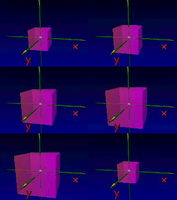
This example is similar, but the transformation is from R³ to itself, and now we'll call it L(x) = 2x. [Click on reload again!]. The yellow interval has been replaced by a pink cube. The corner nearest to us is the vector v = [1,1,1], which moves to L(v) = [2,2,2]. The matrix representation of L is the matrix "M" such that L(v) = Mv [for all v.] Here M=2I, or

You can easily check that M[1,1,1] = [2,2,2] - as it should. Matrices like M are used in most 3D computer graphics programs, and you'll see linear algebra vocabulary even in 2D software like Photoshop.

By the way, "3D graphics" has to be changed to "2D graphics" before it can be put on paper or a monitor. This is (approximately) a special kind of linear transformation from R³ to R², called a projection operator (an "operator" is basically the same thing as a "transformation").

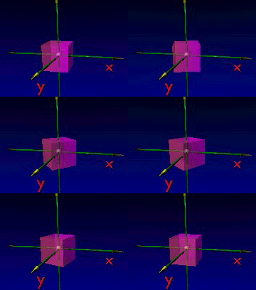
Reload again! This is a picture of a rotation operator. This one goes around the upward z-axis (or the "x₃-axis"). This means, for example, that L(e₃) = e₃. So, e₃ is an eigenvector of L, more on that in Ch 6!

Let's find L's matrix, "M". Notice that e₁ (on the x₁- axis) swings around behind to -e₂, so M[1,0,0] must be [0,-1,0]^T. But M[1,0,0] = the first column of M. Likewise, the second column must be L(e₂), which is e₁. The third column is L(e₃) = e₃. So,

You may want to check that this works; that M e₁ = - e₂, for example. Or (observing the nearest corner) that M[1,1,1] = [1,-1,1]^T. You might have noticed that doing L four times takes us back to the start. That means multiplying any v by M four times should have no effect. So, M⁴ = I. Check this, too! See My Favorite Matrices for more examples like M.

Of course, linear transformations are much more than this. Most of them, such as the familiar derivative operator, L(f)=f ', have little to do with 3D space. But if V has a finite basis, L always has a matrix, which usually helps us understand L.

Read this over a few times, but don't assume that you know it all yet! I haven't scratched the surface!

Back to the Help page